Stop Fighting Messy Tables: Why We Split PDF Table Extraction Across 6 Agents and a Codegen Step
Table of Contents
Extraction demos are easy. We can build one in an afternoon, and so can anyone. Clean document in, clean JSON out, everyone’s impressed. Production is a different animal. The documents you’ve never seen, the layouts built for human eyes, the hundred-page statements that blow past LLM output context token limits, the 99%-isn’t-good-enough math of a workload pushing thousands of documents a day.
That’s the gap between a “wow” and a system that a business can rely on day in and day out. This is where we’ve spent the last couple of years. Here’s how we bridged the gap.
Complex tables don’t faze us humans. We glance at a cramped, chaotic layout and our brains quietly untangle it, finding the patterns and meaning without breaking a sweat. It doesn’t feel like a lot of work, until you try to get a machine to do the same thing. Only when we try to get a LLM to extract data from these tables do we understand actually how difficult it is to do. Even frontier models struggle for complex tables. In this blog, we will discuss how we built our table extractor service which uses 6 agents and a code generation step to do this magic.
The goal
At its core the service is a single function: you hand it a document and a description of what you want, and it hands back clean structured data.
The inputs
The document: a PDF, Excel document or a scanned image
The table class: e.g. bank statement, rent roll
Output schema: the structure you want back, as JSON
Post-processing notes (optional): any transforms to apply
The outputs
Structured data: a JSONL with one record per row
Provenance metadata: highlighting/source data per row, for human eval when needed
Synthetic columns (bonus): new calculated columns derived via post-processing
The real world breaks traditional extraction
The real world contains documents which are messy and designed for humans to read. Not machines. Let’s look at some examples.
One document type, a thousand layouts
A business processing bank statements or rent rolls won’t see one format : it will see hundreds. Every bank and financial institution designs its statements its own way, so the edge cases aren’t a handful but they’re the norm. A rural bank in the US might produce something that barely resembles a “statement” at all. Rent rolls are worse. Not only does every property manager lay them out differently, they each invent their own vocabulary, right down to the column names. We’ve seen it all. The extractor has to handle every one of them, transparently.
Length of tables
A year long bank statement or an agency which handles thousands of properties will have tables that are really long. For example if the statement is a hundred pages long, it is not possible to just pass all the pages in one go to an LLM. There are a few issues here:
An LLM might have a million token input context. But what is not openly advertised is the output context limits. The total output which can be generated is often a fraction of the input context size. This means that we cannot just output the extracted tables directly in these cases. We need to manage the output by doing multiple passes.
Even on the input side, though the input context size for an LLM can be a million tokens, in reality they suffer from a problem called “lost in the middle”. It is a known fact that LLMs are not very good at extracting or considering data in the middle of a large context. This is a critical flaw for table extraction as all the data is equally important.
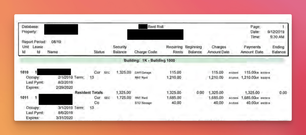
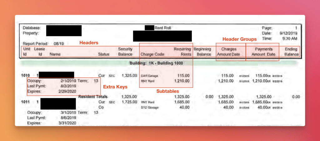
Table designs for human consumption
Some of the layouts we’ve run into are built for exactly one kind of reader: a human eye. Feed them to an LLM with traditional methods and it falls apart. A few examples:
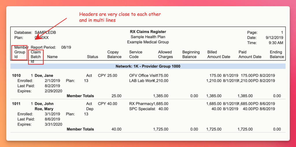
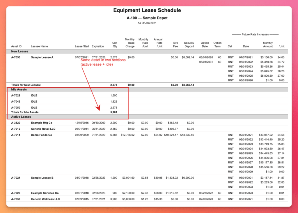
Close headers and offsets
Non standard representations and mixing of contexts within rows: Subtables
Stop wrestling with complex tables — See how LLMWhisperer parses them
The layout-preserved text that feeds our agent pipeline comes from LLMWhisperer. Try it on your own messy PDFs — bank statements, rent rolls, multi-header tables, cross-page rows — No signup required.
Try LLMWhisperer for free on the Playground. No signup required.
Why not a single autonomous agent driven by a powerful LLM?
Let’s get the obvious solution out of the way first. In principle, we could hand a single autonomous agent a powerful frontier model, enough tokens, and enough time. And it would most likely extract even complex tables in the structure we want. But time and again, our customers simply can’t go this route.
That approach is fine for a one-off: personal use, a research project. It falls apart under repetitive, high-volume workloads like bank statements and rent roll processing. The cost per run is very high. In some cases costlier than paying a human, and latency can stretch to minutes per document. For a business pushing thousands of documents a day, it’s a non-starter.
So we built a table extractor that runs at a cost and speed those workloads can actually afford. After all, project viability is one of the most important factors for any workflow automation.
A team of agents instead
Divide and conquer: that’s the approach. Instead of one agent doing everything, we use a team of specialized agents that run one after another. Each taking the table processing a step further and adding its own piece of value.
The reason for splitting it up goes deeper than tidiness. Even frontier models follow complex instructions unreliably once you ask too much of them in a single call. Pile it on (read this messy table, infer its structure, reformat the cells in a certain way and reshape it into my schema, all at once) and the model quietly starts getting things wrong. So we never push the LLM to the edge of its capacity.
Each agent is tasked with achieving exactly one, well-bounded objective that sits comfortably inside the model’s reliability range. For example: we deliberately do not ask the LLM for the user’s final format. We coax it to pull the data out generically, in the language already embedded in the table, and defer the mapping to a later, deterministic stage (the codegen step). Each agent/model does the part it is genuinely good at, and nothing more.
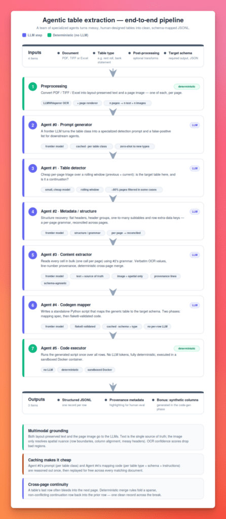
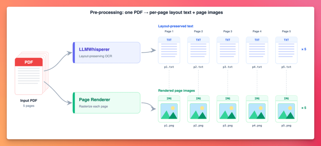
1. Preprocessing : Extracting pages
The first stage in the pipeline is to convert the input document into formats understandable by the LLM. The preprocessing stage produces two sets of artefacts:
Layout-preserved text: one text document per page. (That per-page split matters. We’ll come back to why.)
A page image — one rendered image per page.
We end up with n single page text documents and n images for a n page input document.
2. Agent #0 : Bootstrap prompt generator
Zero-shot generalization to new document types.
The user tells us the table class they’re extracting : “rent roll,” “bank statement,” and so on. Frontier LLMs already know a great deal about these document types, so we put that knowledge to work. A SOTA model writes the specialized prompts the downstream agents will run on.
For example, for Agent #1 It produces a detection prompt. A markdown doc describing the table’s visual characteristics, plus 3–5 false-positive table types to ignore so the detector doesn’t chase look-alikes. And since the same class shows up over and over, the generated prompt is cached and replayed for every future document of that type.
Here’s a sample Agent #0 produced for “rent roll”:
## Target Table: Rent Rolls

### What are Rent Rolls?
Rent Rolls are tables that list individual rental units or tenants in a property, showing current occupancy status, lease terms, and rent amounts for each unit. They provide a snapshot of rental income and tenant information for a property or portfolio.

### Identifying Characteristics
- Column headers typically include: Unit/Suite Number, Tenant Name, Lease Start/End Date, Square Footage, Monthly/Annual Rent, Lease Status (Occupied/Vacant)
- Multiple rows representing individual units or tenants (not aggregated summaries)
- Rent amounts shown per unit (not totals only)
- May include occupancy status indicators or vacancy information
- Often contains lease expiration dates or term lengths for each tenant

### False Positives to Ignore
- Operating expense summaries or budget tables (showing property-level costs, not unit-level rents)
- Rent comparables or market survey tables (showing other properties' rents, not the subject property's actual tenants)
- Income statements or financial summaries (showing aggregated revenue categories, not individual unit details)
- Lease abstract summaries (narrative lease terms without unit-by-unit rent listing)
- Property information sheets or fact sheets (general property details without detailed tenant roster)
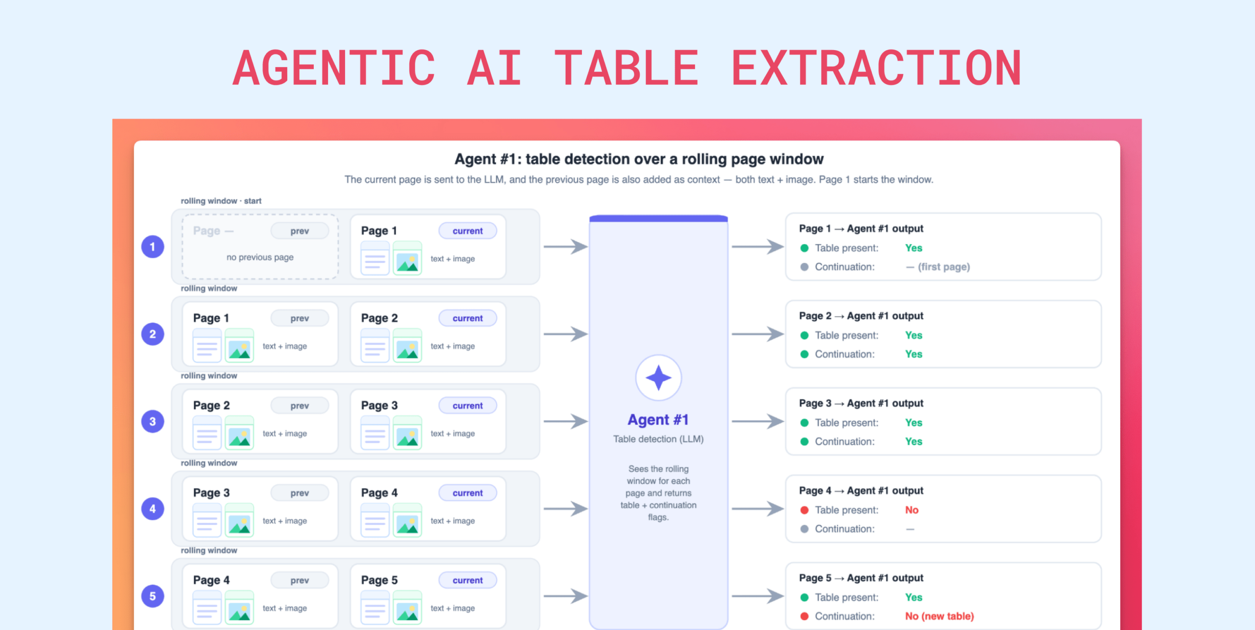
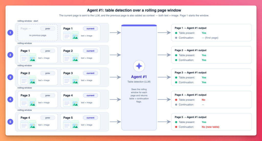
3. Agent #1 : Table presence detector
Up to 80% cost reduction on page filtering. Expensive analysis runs only on relevant pages that actually contain the table we want to extract.
We do a cheap triage with a small, inexpensive model. “Is the target table on this page? Is the table a continuation from the previous page? “. The more expensive models downstream never touch irrelevant pages. Big win!
How to turn complex document tables into usable data with AI
Catch the recorded webinar to dive into Unstract’s advanced table extraction capabilities. We walk through the All Table Extractor API—a ready-to-use, semantic + layout-aware solution that ensures precision, consistency, and context, even across the most complex document tables.
Auditable extraction with full provenance. Every output value is traceable to its source line. Handles the complex, real-world tables that break other extraction tools.
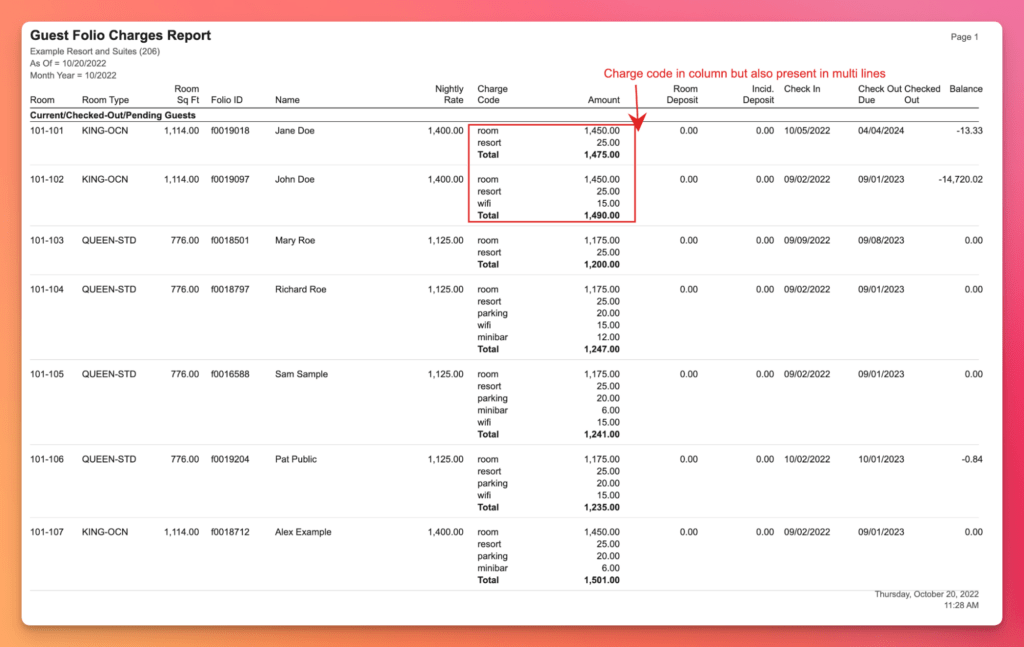
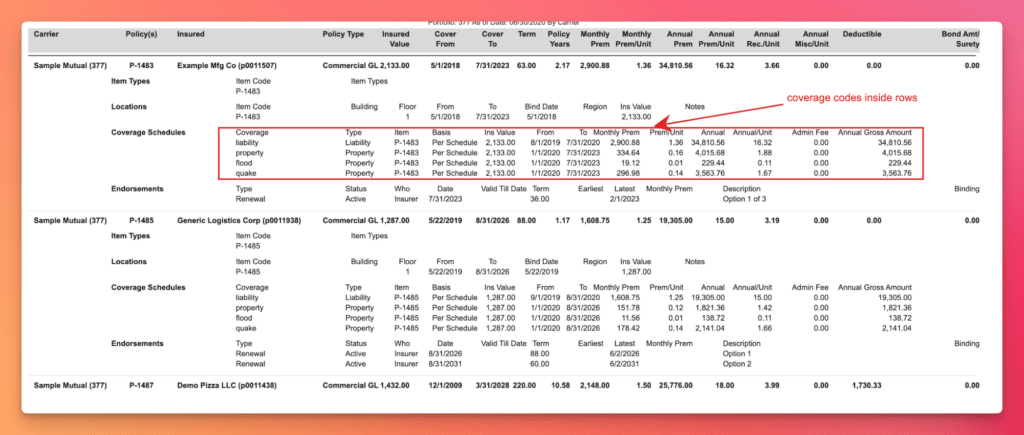
This is the read stage. It takes the structure Agent #2 already discovered (the headers, the one-to-many Charge Code subtable, the Occupy/Term/Expires extra-data keys) and fills it in with actual data.
Because the shape is already known, the LLM spends its effort reading values rather than re-deciding the table’s layout on every page. It reads every cell, but in bulk: one call per page, not cell by cell, emitting rows keyed by the document’s own headers. The result is a generic table, deliberately agnostic to the final output schema.
We send the model both the page image and the layout-preserved text, but the text is the sole source of truth. The prompt tells it to use the image only to settle spatial questions: row boundaries, column alignment, and other layout nuances.
No reshaping or reformatting happens here and the values come out as verbatim OCR strings. "1,105.00" keeps its comma, "5/17/2019" stays raw text, "Cur SEC" stays a raw code. The agent populates the subtable stacked under each unit (when there is one) and the embedded key-value metadata, stamps every row with its OCR line numbers for provenance, and stitches rows across page breaks with a deterministic merge rule.
Real-world tables are messy in structural ways too. One of the most common failure modes for simple extractors is a table whose last row on a page bleeds into the next, where it continues. Solving that reliably at scale isn’t easy. We wrote deterministic rules that fold a sparse, non-conflicting continuation back into the prior row, producing the clean, single-record representation we need.
Any target schema, any mapping logic. An expert Python coding agent writes scripts to do it.
This is the stage where we generate Python code to map the generic extracted table into the structured format the user actually wants. Up to this point, everything we’ve collected stays faithful to the original document: the headers and keys all follow the language and vocabulary of the source table. This stage writes code that deterministically translates that original shape into the user’s target format.
It’s a two-phase approach to schema transformation:
Phase 1 analyzes the user’s target JSON schema alongside the raw extracted structure and produces a complete mapping specification: field names, type conversions, and nested-structure handling.
Phase 2 generates purpose-built Python transformation code and validates it with static analysis (flake8). If validation fails, it self-corrects from the error feedback.
Concretely: it feeds the target schema, any user instructions, and a small (~3 row) sample of Agent #3’s generic table into a meta-prompt that writes the actual code-generation prompt. That prompt then emits a single standalone, stdlib-dependent-only Python script that reads the extracted rows and writes the target JSONL. The script is where the mapping lives: reusable rules that turn "1,105.00" into a number, "5/17/2019" into a normalized date, "Cur SEC” into an occupancy status, Occupy into move_in, and the stacked Charge Code subtable into clean line items.
Because the code is written once and applied identically to every row, a parsing rule is right-or-wrong globally rather than stochastically per row. The script is flake8-validated, and regenerated with the errors fed back in if it fails.
It’s then cached on the table type, schema, and instructions, so this expensive reasoning happens once per schema and is replayed for free across every matching document. The model interprets the table’s shape a single time and freezes the result as code. Nothing here runs per row, and no document’s values are ever touched. That’s deferred to the executor agent.
Bonus: synthetic columns
Because the mapping is code, we can add synthetic columns: columns computed from other columns or from arbitrary logic. It’s a powerful lever that can eliminate downstream steps entirely. A synthetic column can be as simple as a formula over existing fields, or as involved as a validity check that decides whether a row satisfies a set of constraints.
A sample target format
A rent roll processing office typically handles rent rolls from hundreds of customers, each with its own formatting and vocabulary (the example from the previous agents is one such case). For downstream processing to work, all of that extracted data has to land in one common shape. That common shape is what this mapping produces.
Because the extracted data still speaks the document’s language, not the user’s. Every rent roll labels and formats things its own way, but downstream systems expect one consistent shape. Mapping bridges the two: it turns each document’s native vocabulary and quirks into the standard schema the user needs.
User required
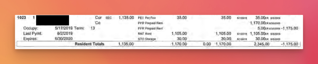
Document vocabulary and format
unit_num: “1023”
“Unit Id”
occupancy: “Occupied” (enum)
“Status”: “Cur SEC” (raw code)
move_in: “2019-05-17” (date)
“Occupy”: “5/17/2019”
lease_end: “2020-06-30”
“Expires”: “6/30/2020”
rent_charge: 1105.0 (number)
“RNT Rent” / “1,105.00” line in the Charge Code subtable
charge_codes: [{code, amount}]
Subtables “Charge Code” with {Charge Code, Recurring Rents}
None of that mapping : renaming fields, “Cur SEC” → “Occupied”, “5/17/2019” → “2019-05-17”, “1,105.00” → 1105.0, flattening the subtable exists anywhere in the pipeline until Agent 4 reads this schema and writes a python script to do it.
Turn your complex PDF tables into structured data with Unstract
Unstract uses LLMs to extract clean, structured JSON from any document — PDFs, scans, images, tables of any layout. Define what you want using natural language, deploy as an API or ETL pipeline, and get data your systems can actually use.
Try Unstract for free on the Playground. No signup required.
Sandboxed execution. Enterprise-grade security. The generated code never touches network or other data
This is the run stage, and it makes no LLM calls at all. It takes the Python script Agent #4 produced and runs it once over the entire set of extracted rows. No matter how many rows there are, zero LLM tokens are spent. Because the logic is now ordinary code, the same input yields deterministic, identical output on every run. The LLM’s job is already done. Execution is sandboxed: by default the script runs in a throwaway Docker container.
Special technique used to increase reliability
We send the LLM both the layout-preserved text and an image of the page. Our system prompts tell it to use the image as a spatial reference for the page’s organization, and to always treat the layout-preserved OCR text as the single source of truth. This split has two real benefits:
The OCR step gives us deterministic confidence scores, which we can use to drop bad sections or words before they ever reach the model.
For a multimodal LLM, the image is a valuable spatial signal, especially on tables with complex layouts or bad, malformed header spacing.
Multi-Agent PDF Table Extraction Pipeline: Wrapping up
Complex tables are trivial for a person to parse but brutal for a single agent trying to do everything at once in a single LLM call. Our solution was to stop asking one model to do it all.
By splitting the work across a team of specialized agents, each one cheap to run and good at exactly one job of well-defined scope, we get extraction that survives the real world: hundreds of layout variants, hundred-page documents, and tables built for human eyes.
The decisions that make it production-ready are threaded throughout the pipeline. Cheap triage, so the expensive models only ever see relevant pages. Structure recovered once, then reused. Mapping frozen into deterministic code instead of re-reasoned per row.
Prompts and code cached per document class, so the costly thinking happens once and replays for free. Verbatim values and line-number provenance, so every output traces back to its source.
If there is one idea to take away, it is this: we never ask the LLM for more than it can reliably give. Each agent uses just enough of the model and no more, and everything that can be made deterministic is pushed out of the model and into code (that the agents themselves generate).
That is what turns a “wow” demo into something that runs at a cost, accuracy, reliability and latency a business can live with, even at thousands of documents a day.
If you are fighting messy tables, that is exactly what we built Unstract and LLMWhisperer to handle.
Multi‑Agent PDF Table Extraction: FAQs
1. Why does a single autonomous LLM agent fail for production‑grade table extraction? A single agent with a powerful frontier model can extract complex tables for one‑off use, but it becomes too slow and expensive for high‑volume workloads like bank statements or rent rolls. Latency stretches to minutes per document and cost per run can exceed paying a human, making it a non‑starter for businesses processing thousands of documents daily.
2. How does the 6‑agent pipeline handle hundred‑page documents without hitting output context limits? The pipeline splits the document page‑by‑page and uses Agent #1 (Table presence detector) as a cheap triage to filter out irrelevant pages. Only pages that actually contain the target table reach the more expensive models, reducing cost by up to 80% and keeping per‑page content manageable.
3. What is the role of Agent #0 (Bootstrap prompt generator) in the pipeline? Agent #0 uses a frontier LLM to generate specialized prompts for downstream agents based on the user’s table class (e.g., “rent roll” or “bank statement”). These prompts are cached and replayed for every future document of that type, so the expensive reasoning happens once per document class.
4. How does Agent #4 (Codegen, master data mapper) improve reliability over direct LLM schema mapping? Agent #4 writes a standalone Python script that deterministically maps the generic extracted table into the user’s target JSON schema. Once validated with flake8 and self‑corrected, the script is cached and applied identically to every row – turning stochastic per‑row reasoning into deterministic, bug‑free transformations.
5. How does the pipeline ensure every extracted value is auditable and traceable? Agent #3 (Content extractor) stamps every row with its OCR line numbers (provenance metadata) during extraction. This allows any output value to be traced back to its exact source line in the original document, which is critical for human evaluation and compliance.
6. What special technique does the pipeline use to improve reliability on complex table layouts? The pipeline sends both layout‑preserved OCR text and a page image to the LLM during extraction. The system prompt instructs the model to use the image only for spatial reference (row boundaries, column alignment) while treating the OCR text as the single source of truth – combining the strengths of both modalities.
UNSTRACT
AI Driven Document Processing
The platform purpose-built for LLM-powered unstructured data extraction. Try Playground for free. No sign-up required.